Blogs

While DF is still an important avenue for speeding calculations today, a couple of factors made it invaluable at the advent of computational chemistry. The first of these was the use of Slater type orbitals (STOs) in early chemistry software. STOs are close approximate solutions of the Schrödinger equation and as such were a clear choice for early basis sets. Despite this accuracy, the great shortcoming of STOs is that products of more than two STOs lead to expressions that are impossible to integrate analytically. This is in contrast to the most popular type of orbital used now, the Gaussian type orbital (GTO), which when multiplied with another GTO gives another translated GTO, which in turn can be readily integrated analytically. This necessitated the use of approximation techniques or semi-empirical parameters in STO calculations involving more than two centers. The other big factor is a bit more obvious but still important: old computers were slower and more expensive to operate. This means that numerical integrals were often too expensive or time-consuming to compute, which compounds the lack of analytic forms for the multi-center STO integrals.

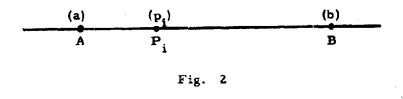
With this in mind, one of the earliest studies on a triatomic molecule necessitated the development of an early DF technique that involved expanding two-center charge distributions by a least-squares procedure as a sum of single-center charge distributions centered on a line passing through the two centers. This sounds complicated, but the main idea is summarized readily by Fig. 2 from the paper Boys and Shavitt (1959) reproduced below:

Similarly, the corresponding mathematical expression is given by the equation

\begin{equation} ab \cong \sum_{i}^m C_i p_i, \end{equation}

where the \(p_i\) are a uniform set of 20 symmetrically placed exponential functions and the \(C_i\) are coefficients adjusted to minimize the metric

\begin{equation} \int(ab - \sum_p C_{i}p_i)d\tau, \end{equation}

which is just the previous equation rearranged and integrated over the set of two-center charge distributions \(ab\).

Basically, the authors approximate the difficult integrals by a linear combination of primitive exponential functions. If you are familiar with the STO-nG basis sets, and really any modern Gaussian basis sets, this should sound quite familiar. The authors are essentially describing a STO-20E basis set, where they approximate an STO as a contraction of 20 exponential functions rather than n Gaussian functions. This should serve as a clear indication of the difficulty of the integrals themselves since the authors are willing to increase the number of terms by a factor of 20 to obtain easier computations.

Seven years later, in 1966, the same problems with STOs persisted, and many more methods had been proposed to treat the necessary integrals approximately by people you have probably heard of. Mulliken, for example, proposed approximating a two-center orbital product by the simple average of the single-center orbitals involved. Löwdin made the rather straightforward suggestion to extend this by taking the weighted average to preserve the correct dipole moment. These and many more are described by Harris and Rein, but the takeaway is that all of these methodologies can be seen as taking the leading terms from infinite series expansions of the two-center charge densities, much like Boys and Shavitt did. The goal of the authors then was to use this perspective, combined with a new procedure for optimizing the coefficients of the charge densities, to yield the most accurate approximation scheme to date.

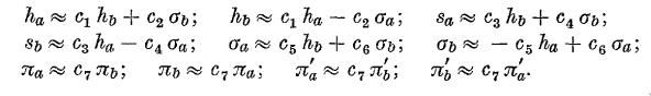
Their general scheme was to expand orbitals about one center in a series about the other center using terms of each atomic symmetry, where at least in this paper they have restricted themselves to \(s\) and \(p\) symmetry as you can see in the figure below. They use \(h\) to denote a 1\(s\) orbital, \(s\) for 2\(s\), \(\sigma\) for the \(m=0\) 2\(p\) orbitals, and \(\pi\) for the \(m=\pm1\) 2\(p\) orbitals. The prime indicates the negative version.

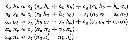
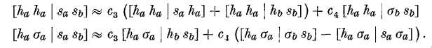
Using these definitions, the products of the orbitals can be written as

and

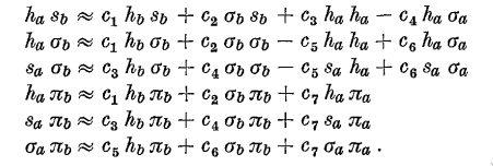
The rather primitive fitting is done by taking pairs of integrals involving the same coefficients and solving the resulting linear system, as shown in the example below, where \(c_3\) and \(c_4\) are being determined.

Once the coefficients are determined, the difficult, four-center electron repulsion integrals can then be computed as linear combinations of the much easier one-center integrals and two-center Coulomb integrals. As the authors point out, this procedure requires integrals on only \(\frac{n(n-1)}{2}\) pairs of centers compared to the \(n^4\) needed for the full computation, and they achieve accuracies relative to the exact integral calculations of 1 kcal.

By 1971 the use of GTOs had become more widespread following the introduction of the STO-nG basis sets by John Pople in 1969, but there are some downsides of using GTOs as well. The chief among these is the fact that GTOs have improper limiting behavior at both the nucleus, where they are rounded instead of forming a cusp, and at long range, where they decay too quickly. However, these issues can be mitigated by taking linear combinations of multiple primitive Gaussian functions to form something more closely resembling an STO. As such, most modern software instead uses this type of GTOs where multiple individual Gaussians are contracted into something that can more closely emulate the limiting behavior of STOs. This practice is most obvious in the naming of the aforementioned STO-nG basis sets, which form approximate STOs from contractions of n primitive (G)aussian functions. Another problem is that this contraction scheme introduces a potentially large number of GTOs relative to the number of STOs required, but now at least the integrals can be evaluated analytically. Nevertheless, numbers were larger in the 1970s relative to the available computer power, so reducing the number of integrals by decomposing them into reusable pieces was the problem Billingsley and Bloor sought to address in their work on the limited expansion of diatomic overlap (LEDO) approximation. While this may sound somewhat different from the earlier problem, this begins to illustrate the wide application of the density fitting technique.

Another deficiency Billingsley and Bloor pointed out in the earlier work, including that of Harris and Rein, was the lack of full symmetry handling in the approximate two-center charge distributions. For example, in the Harris and Rein formulation, using only one 1\(s\) and 2\(p\) orbital for the approximations leads to missing irreducible representations of the rotation groups for the orbitals with \(p\) symmetry. This leads to incorrect or missing nodal structures in the resulting approximate distributions. To remedy this, Billingsley and Bloor suggested the following definition for the two-center charge distribution \(\pi_k^{AB}\):

\begin{equation} \pi_k^{AB} \cong \sum_p^{\text{on }A}C_{kp}\Omega_p^A + \sum_q^{\text{on }B}C_{kq}\Omega_q^B \end{equation}

where \(\Omega_p^A\) is a unique one-center distribution formed by the product of two orbitals, \(\chi_m^A\chi_n^A\). This gives a set of approximate two-center charge distributions as a linear combination of the one-center distributions inherent in the basis set of choice since we are summing over the unique sets of one-center distributions on the two atomic centers in question. This has the additional benefit of generalizing immediately to any set of AO basis functions. With this formulation in hand, the authors now needed to determine the \(C\) values. Because of the success of the Harris-Rein approach there, they maintained the same approach of fitting the coefficients to a relatively small set of exact integrals but introduced a matrix notation more appropriate for the larger systems of equations involved.

The fundamental equation here is

\begin{equation} (\Omega_i^A | \frac{1}{r_{12}} | \pi_k^{AB}) \cong \sum C_{kp}(\Omega_i^A| \frac{1}{r_{12}} | \Omega_p^B), \end{equation}

where you can use the definitions

\begin{equation} L_{ij} \equiv (\Omega_i^A | \frac{1}{r_{12}} | \pi_j^{AB}) \end{equation}

and

\begin{equation} J_{ip} \equiv (\Omega_i^A| \frac{1}{r_{12}} | \Omega_p^B), \end{equation}

to rewrite the problem as the matrix expression

\begin{equation} \boldsymbol{L} = \boldsymbol{CJ}, \end{equation}

which can be solved for the coefficients by inverting \(\boldsymbol{J}\). The authors point out that this inversion can be quite touchy due to the often ill-conditioned \(\boldsymbol{J}\) matrix, so care must be taken in performing it. However, the resulting coefficients can be used in Eqn. 4 to yield the full set of two-center charge distributions, which in turn are used to generate three- and four-center integrals by taking linear combinations of the one- and two-center Coulomb and hybrid integrals. The agreement produced by the LEDO method is only 12.5 kcal/mol relative to full integral calculations, but as the authors point out, this cannot be compared directly to the results of Harris and Rein, who only looked at homonuclear diatomics, whereas Billingsley and Bloor examined a test set including polyatomic molecules like formaldehyde, methane, acetylene, and ethylene.

According to Reine, et al., the modern version of density fitting was introduced independently by J. L. Whitten and Baerends, et al. in 1973, shortly after the developments of Billingsley and Bloor. The basic idea in both of these formulations was to embed the fitting procedure in the definition of the approximated densities. In Whitten's words, the goal was "to relate the method of determination of approximate densities directly to the error bound," in contrast to the previous work which proposed some form for the approximate densities and then imposed an external metric for the optimization. Whitten, in particular, sought a definition of the approximate densities based on a definition of the error bound on the approximation, leading to a clear path to optimization. For Whitten the error bound of interest was

\begin{equation} |[\phi_a(1) | r_{12}^{-1} | \phi_b(2)]-[\phi_a'(1) | r_{12}^{-1} | \phi_b'(2)]| \leq \delta, \end{equation}

where the primes indicate the approximate versions of the exact one-particle charge densities \(\phi_a\) and \(\phi_b\). By a series of proofs, Whitten demonstrates that minimization of the quantity

\begin{equation} \epsilon_a = [\phi_a(1) - \lambda_a\phi_a''(1) | r_{12}^{-1} | \phi_a(2) - \lambda_a\phi_a''(2) ] \end{equation}

with respect to \(\lambda_a\) and the parameters of \(\phi_a''\), which is \(\phi_a' / \lambda_a\) also minimizes the error in the approximation, \(\delta\), as was desired. For the four-center electron repulsion integrals this yields the approximation

\begin{equation} \int\phi_i^*(1)\phi_j(1)\frac{1}{r_{12}}\phi_k^*(2)\phi_l(2) \approx \lambda_{ij}\lambda_{kl}[\Phi_{ij}(1) | r_{12}^{-1} | \Phi_{kl}(2)], \end{equation}

where \(\phi_i(1)\phi_j(1)\) is approximated by \(\lambda_{ij}\Phi_{ij}(1)\) and the \(\Phi\)s are of some chosen functional form. Whitten suggests that the interesting choices of \(\Phi\) are either contractions of Gaussian functions, in which you can choose a smaller number of Gaussians \(g_m'\) to represent the full set \(g_m\) and approximate \(\Phi_{mn}\) as \(\lambda_{mn}g_m'g_n'\), or using the expansion \(\Phi_{mn} = \sum_k^Mc_k\Omega_k\), which as Whitten points out is the same as that suggested by Harris and Rein and Billingsley and Bloor. Consequently, Whitten offers a more solid theoretical basis for the work that came before him and formalizes the practice of density fitting.

Now the major differences in implementations of DF arise in the metric used to assess the fitting. Since Whitten's procedure relies on \(\delta\) defined in terms of the Coulomb operator \(r_{12}^{-1}\), his is referred to as the "Coulomb metric." Baerends, et al., on the other hand, introduced what is known as the "overlap metric," where the Coulomb operator is replaced by the overlap operator defined as \(w = \delta(r_1 - r_2\). by the authors this is reminiscent of the LEDO procedure described by Billingsley and Bloor, given that they approximate the density as

\begin{equation} \rho^{AB} = \sum_\mu^A \sum_\nu^B P_{\mu\nu}\chi_\mu^A\chi_\nu^B, \end{equation}

but instead of fitting the full set of \(\chi_\mu^A\chi_\nu^B\), they restrict themselves to a smaller set of \(s\) type STOs, which is somewhat more similar to the original Boys and Shavitt approach. Obviously this selection satisfies the mathematical constraints described by Whitten with the \(s\) type STOs taking the place of the \(\Phi\) functions. Something to point out explicitly here is that these \(\Phi\)s serve as an auxiliary basis in which to carry out the calculation. Rather than working in the original basis with functions on each nucleus, you can reduce the problem conceptually to operating in the auxiliary basis with functions in the space between nuclei.

According again to Reine, not to be confused with Rein of the Harris and Rein work, who reviewed these developments in 2008, later work by Dunlap revealed that the Coulomb metric of Whitten was superior to the overlap metric suggested by Baerends. This is somewhat unsurprising to me given the mathematical rigor of Whitten's approach compared to that of Baerends, et al. However, the Baerends work was trying to solve the more specific problem of computing properties of large molecules for which it was necessary to abandon some rigor. Their approach offered a substantial improvement over the contemporary standard of using semi-empirical methods and the muffin-tin approximation, so it certainly served its purpose. Nevertheless, later work has sought to build on the Coulomb metric as a result of its greater accuracy.

This is where the work of Reine, et al. fits. As they point out in 2008, the development of HF and density functional theory (DFT) procedures that scale linearly made even density fitted integral calculations, which scale cubically in the full Coulomb metric, the slow step in HF and DFT computations. As such, they sought a linear-scaling DF approach to keep up with these faster methods. To achieve this, they built on the local atomic density fitting (LADF) and atomic resolution of the identity (ARI) approaches of Sodt et al., which rely on pruning the auxiliary basis down to those functions that are suitably close to the atoms in question. However, these earlier approaches had relied on the choice of an artifactual "bump" function to implement the pruning. Reine et al. then devised a method of pruning the auxiliary basis that was more robust while maintaining the variational property of the LADF approach. The mathematics are rather involved, so I will defer to the original work for those interested in the details of this "local" fitting metric.

Regardless of the metric, Equation 13 gives the concise definition of density fitting. The choice of \(\Phi\) is the choice of the auxiliary basis to perform the density fitting on, and the metric chosen will affect the fitting procedure or equivalently the determination of the \(\lambda\) values.

Density fitting is often referred to as resolution of the identity (RI) because another way of expressing the approximation in Equation 13 is by the introduction of the RI operator

\begin{equation} I = \sum_m |m)(m| \end{equation}

into the integral

\begin{equation} (ij|kl) = \int\phi_i^*(1)\phi_j(1)\frac{1}{r_{12}}\phi_k^*(2)\phi_l(2) \end{equation}

to produce

\begin{equation} (ij|kl) = \sum_m (ijm)(m|kl) \end{equation}

where the four-center integral has clearly been reduced to the product of a three-center one-electron overlap integral and a three-center, two-electron repulsion integral, as demonstrated by Feyereisen et al. \(m\) denotes an auxiliary basis in the space of \(ij\), which it can either expand completely or approximate via an incomplete expansion. This is useful not only for HF, in which the resulting integrals are used directly, but also in post-HF methods like MP2, which require the transformation of the AO basis into the molecular orbital (MO) basis. If you have done the Crawford programming projects, you will know that even in the best case the MO transformation scales as \(\mathcal{O}(N^5)\) when using the four-center integrals. Using the RI/DF approximation reduces the integrals to three-center integrals and correspondingly reduces the MO transformation to \(\mathcal{O}(N^4)\). Similar improvements can be attained in coupled-cluster computations, as suggested by Rendell and Lee.

Density fitting is a powerful technique for speeding up quantum chemical calculations. Initially it was used to approximate intractable integrals inherent in STO calculations, but it has now been utilized to reduce the number of integrals that must be calculated in computations using large GTO basis sets. Additionally, the RI formalism helps to extend the performance gains of using density-fit integrals to correlated methods like MP2 and coupled-cluster theory, making density fitting an invaluable component of modern theoretical chemistry investigations.